Special Functions
Overview
The special package of Hipparchus gathers several useful special functions not provided by java.lang.Math.
Erf functions
Erf contains several useful functions involving the Error Function, Erf.
| Function | Method | Reference |
|---|---|---|
| Error Function | erf | See MathWorld |
Gamma functions
Class Gamma contains several useful functions involving the Gamma Function.
Gamma
Gamma.gamma(x) computes the Gamma function, \(\Gamma(x)\) (see MathWorld, DLMF). The accuracy of the Hipparchus implementation is assessed by comparison with high precision values computed with the Maxima Computer Algebra System.
| Interval | Values tested | Average error | Standard deviation | Maximum error |
|---|---|---|---|---|
| \(-5 \lt x \lt -4\) | x[i] = i / 1024, i = -5119, ..., -4097 |
0.49 ulps | 0.57 ulps | 3.0 ulps |
| \(-4 \lt x \lt -3\) | x[i] = i / 1024, i = -4095, ..., -3073 |
0.36 ulps | 0.51 ulps | 2.0 ulps |
| \(-3 \lt x \lt -2\) | x[i] = i / 1024, i = -3071, ..., -2049 |
0.41 ulps | 0.53 ulps | 2.0 ulps |
| \(-2 \lt x \lt -1\) | x[i] = i / 1024, i = -2047, ..., -1025 |
0.37 ulps | 0.50 ulps | 2.0 ulps |
| \(-1 \lt x \lt 0\) | x[i] = i / 1024, i = -1023, ..., -1 |
0.46 ulps | 0.54 ulps | 2.0 ulps |
| \( 0 \lt x \le 8\) | x[i] = i / 1024, i = 1, ..., 8192 |
0.33 ulps | 0.48 ulps | 2.0 ulps |
| \( 8 \lt x \le 141\) | x[i] = i / 64, i = 513, ..., 9024 |
1.32 ulps | 1.19 ulps | 7.0 ulps |
Log Gamma
Gamma.logGamma(x) computes the natural logarithm of the Gamma function, \(\log \Gamma(x)\), for \(x \gt 0\) (see MathWorld, DLMF). The accuracy of the Hipparchus implementation is assessed by comparison with high precision values computed with the Maxima Computer Algebra System.
| Interval | Values tested | Average error | Standard deviation | Maximum error |
|---|---|---|---|---|
| \(0 \lt x \le 8\) | x[i] = i / 1024, i = 1, ..., 8192 |
0.32 ulps | 0.50 ulps | 4.0 ulps |
| \(8 \lt x \le 1024\) | x[i] = i / 8, i = 65, ..., 8192 |
0.43 ulps | 0.53 ulps | 3.0 ulps |
| \(1024 \lt x \le 8192\) | x[i], i = 1025, ..., 8192 |
0.53 ulps | 0.56 ulps | 3.0 ulps |
| \(8933.439345993791 \le x \le 1.75555970201398e+305\) | x[i] = 2**(i / 8), i = 105, ..., 8112 |
0.35 ulps | 0.49 ulps | 2.0 ulps |
Regularized Gamma
Gamma.regularizedGammaP(a, x) computes the value of the regularized Gamma function, P(a, x) (see MathWorld).
Beta functions
Beta contains several useful functions involving the Beta Function.
Log Beta
Beta.logBeta(a, b) computes the value of the natural logarithm of the Beta function, log B(a, b). (see MathWorld, DLMF). The accuracy of the Hipparchus implementation is assessed by comparison with high precision values computed with the Maxima Computer Algebra System.
| Interval | Values tested | Average error | Standard deviation | Maximum error |
|---|---|---|---|---|
| \(0 \lt x \le 8\) \(0 \lt y \le 8\) |
x[i] = i / 32, i = 1, ..., 256y[j] = j / 32, j = 1, ..., 256 |
1.80 ulps | 81.08 ulps | 14031.0 ulps |
| \(0 \lt x \le 8\) \(8 \lt y \le 16\) |
x[i] = i / 32, i = 1, ..., 256y[j] = j / 32, j = 257, ..., 512 |
0.50 ulps | 3.64 ulps | 694.0 ulps |
| \(0 \lt x \le 8\) \(16 \lt y \le 256\) |
x[i] = i / 32, i = 1, ..., 256y[j] = j, j = 17, ..., 256 |
1.04 ulps | 139.32 ulps | 34509.0 ulps |
| \(8 \lt x \le 16\) \(8 \lt y \le 16\) |
x[i] = i / 32, i = 257, ..., 512y[j] = j / 32, j = 257, ..., 512 |
0.35 ulps | 0.48 ulps | 2.0 ulps |
| \(8 \lt x \le 16\) \(16 \lt y \le 256\) |
x[i] = i / 32, i = 257, ..., 512y[j] = j, j = 17, ..., 256 |
0.31 ulps | 0.47 ulps | 2.0 ulps |
| \(16 \lt x \le 256\) \(16 \lt y \le 256\) |
x[i] = i, i = 17, ..., 256y[j] = j, j = 17, ..., 256 |
0.35 ulps | 0.49 ulps | 2.0 ulps |
Regularized Beta
(see MathWorld)
Elliptic functions and integrals
Notations in the domain of elliptic functions and integrals is often confusing and inconsistent across text books. Hipparchus implementation uses the parameter m to define both Jacobi elliptic functions and Legendre elliptic integrals and uses the nome q to define Jacobi theta functions. The elliptic modulus k (which is the square of parameter m) is not used at all in Hipparchus. All these parameters are linked together.
See in MathWorld elliptic integrals of the first kind, elliptic integrals of the second kind, elliptic integrals of the third kind, Jacobi elliptic functions and Jacobi theta functions.
JacobiEllipticBuilder.build(m) builds a JacobiElliptic (or FieldJacobiElliptic) implementation for the parameter m that computes the twelve elliptic functions \(sn(u|m)\), \(cn(u|m)\), \(dn(u|m)\), \(cs(u|m)\), \(ds(u|m)\), \(ns(u|m)\), \(dc(u|m)\), \(nc(u|m)\), \(sc(u|m)\), \(nd(u|m)\), \(sd(u|m)\), and \(cd(u|m)\). The functions are computed as copolar triplets as when one function is needed in an expression, the two other are often also needed. The inverse functions \(arcsn(u|m)\), \(arccn(u|m)\), \(arcdn(u|m)\), \(arccs(u|m)\), \(arcds(u|m)\), \(arcns(u|m)\), \(arcdc(u|m)\), \(arcnc(u|m)\), \(arcsc(u|m)\), \(arcnd(u|m)\), \(arcsd(u|m)\), and \(arccd(u|m)\) are also available.
JacobiTheta (and FieldJacobiTheta) computes the four Jacobi theta functions \(\theta_1(z|\tau)\), \(\theta_2(z|\tau)\), \(\theta_3(z|\tau)\), and \(\theta_4(z|\tau)\). The half-period ratio \(\tau\) is linked to the nome q: \(q = e^{i\pi\tau}\). Here again, the four functions are computed at once and a quadruplet is returned.
CarlsonEllipticIntegrals is a utility class that computes the following integrals in Carlson symmetric form, for both primitive double, CalculusFieldElement, Complex and FieldComplex:
| Name | Definition |
|---|---|
| \(R_F(x,y,z)\) | \(\frac{1}{2}\int_{0}^{\infty}\frac{\mathrm{d}t}{s(t)}\) |
| \(R_J(x,y,z,p)\) | \(\frac{3}{2}\int_{0}^{\infty}\frac{\mathrm{d}t}{s(t)(t+p)}\) |
| \(R_G(x,y,z)\) | \(\frac{1}{4}\int_{0}^{\infty}\frac{1}{s(t)}\left(\frac{x}{t+x}+\frac{y}{t+y}+\frac{z}{t+z}\right)t\mathrm{d}t \) |
| \(R_D(x,y,z)\) | \(R_J(x,y,z,z)\) |
| \(R_C(x,y)\) | \(R_F(x,y,y)\) |
where \(s(t) = \sqrt{t+x}\sqrt{t+y}\sqrt{t+z}\).
LegendreEllipticIntegrals is a utility class that computes the following integrals, for both primitive double, CalculusFieldElement, Complex and FieldComplex. (the implementation uses CarlsonEllipticIntegrals internally):
| Name | Type | Definition |
|---|---|---|
| \(K(m)\) | complete | \(\int_0^{\frac{\pi}{2}} \frac{d\theta}{\sqrt{1-m \sin^2\theta}}\) |
| \(K'(m)\) | complete | \(\int_0^{\frac{\pi}{2}} \frac{d\theta}{\sqrt{1-(1-m) \sin^2\theta}}\) |
| \(E(m) \) | complete | \(\int_0^{\frac{\pi}{2}} \sqrt{1-m \sin^2\theta} d\theta\) |
| \(D(m) \) | complete | \(\frac{K(m) - E(m)}{m}\) |
| \(\Pi(n, m)\) | complete | \(\int_0^{\frac{\pi}{2}} \frac{d\theta}{\sqrt{1-m \sin^2\theta}(1-n \sin^2\theta)}\) |
| \(F(\varphi, m)\) | incomplete | \(\int_0^{\varphi} \frac{d\theta}{\sqrt{1-m \sin^2\theta}}\) |
| \(E(\varphi, m)\) | incomplete | \(\int_0^{\varphi} \sqrt{1-m \sin^2\theta} d\theta\) |
| \(D(\varphi, m)\) | incomplete | \(\frac{K(\varphi, m) - E(\varphi, m)}{m}\) |
| \(\Pi(n, \varphi, m)\) | incomplete | \(\int_0^{\varphi} \frac{d\theta}{\sqrt{1-m \sin^2\theta}(1-n \sin^2\theta)}\) |
Beware that when computing elliptic integrals in the complex plane, many issues arise due to branch cuts. One typical example is the integral \(\Pi(n, \varphi, m)\), which is defined as \[ \Pi(n, \varphi, m) = \int_0^{\varphi} \frac{d\theta}{\sqrt{1-m \sin^2\theta}(1-n \sin^2\theta)} \] \(\varphi\) is the amplitude, \(n\) is the elliptic characteristic, \(m\) is the ellipse parameter (some conventions use the elliptic modulus \(k\) such that \(m=k^2\) instead of the parameter \(m\), or they use the nome \(q\)). All variables that appear in this expression may be complex.
The integrand has poles corresponding to \[ \theta_m = \pm \arcsin\frac{1}{\sqrt{m}},\quad\theta_n = \pm \arcsin\frac{1}{\sqrt{n}} \] and their periodic repetitions due to the inverse sines.
The integral is expected to be computed over the straight path from \(0\) to \(\varphi\). With this assumption, the integral is a single-valued function. The following picture shows the value of the integral for \(n=3.4-1.3i\) and \(m=0.2+0.6i\).
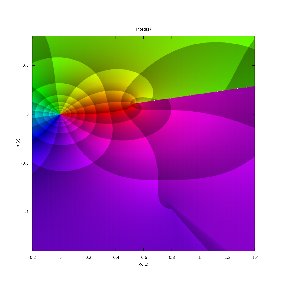
One can clearly see the pole near \(0.537+0.110i\) as the start point of a ray separating a green and a purple zone. Domain coloring uses hue to represent phase plus periodic brightness to enhance both modulus and phase. The sharp green/purple transition on the right hand side shows there is a discontinuity when crossing this ray. There is another pole (less visible) near \(0.785-0.909i\) and another ray. Drawing the integral on a larger range would show other rays dues to the repetitions of these poles.
If we take care to never cross the rays cast by poles, we could in fact compute the integral using other paths than the straight line from \(0\) to \(\varphi\). We could for example start parallel to the real axis and then parallel to the imaginary axis, or any other path.
If on the other hand we compute the integral using a path that crosses these rays (i.e. a path that goes after the poles and then bends upwards or downward before reaching \(\varphi\), then we don't notice that we cross the rays because in fact there are no poles along the path, the poles are really isolated. So in this case, we compute a value of the integral that is finite and looks perfectly reasonable, but is different from the value that would be computed by the straight path. The following example shows one example of the results we could obtain.
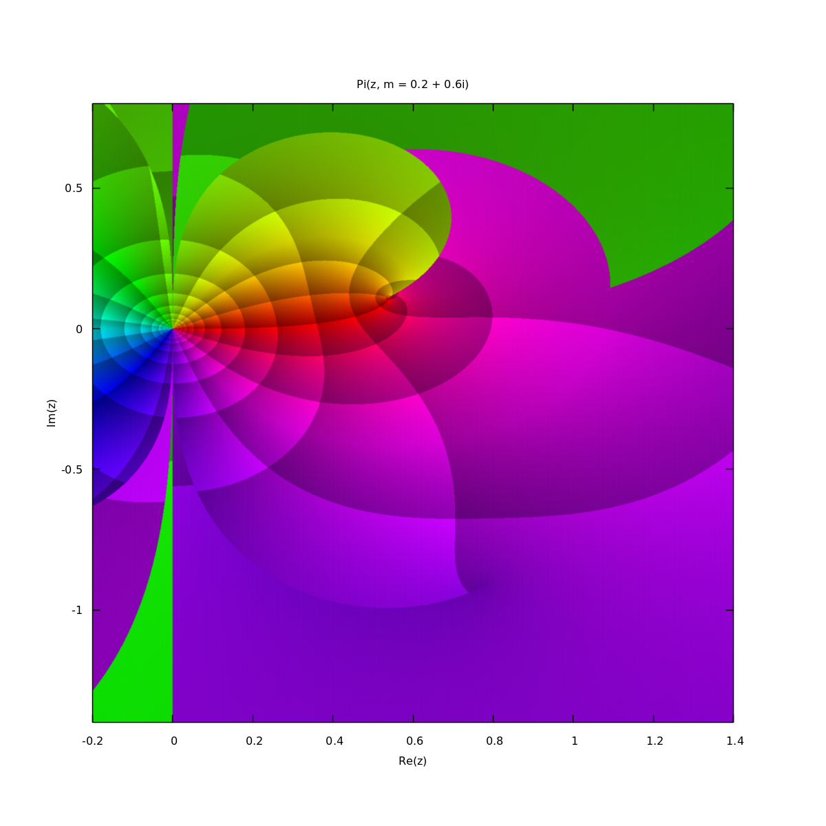
We see that the purple region extended upwards in a wave-like shape. In fact, we have chosen a different sheet of the Riemann surface that represent the integral value.
The first image was really computed using numerical integration. The second image was in fact computed using the Carlson transformation that allows much faster results.
Numerical integration is not only very slow, it sometimes fails to converge. The tiny white points on the ray cast by the first pole correspond to failures: the integrator exceeded its maximum number of iterations (despite it was huge). The lower ray is also in fact probably false numerically, there should be a more pronounced color change, here we seem to just have some darker purple which we think is wrong.
Carlson transformations are extremely fast, but they obviously select the wrong value without notice. The changes occur when during internal iterations we compute a value \(\lambda_m=\sqrt{x_m}\sqrt{y_m}+\sqrt{x_m}\sqrt{z_m}+\sqrt{y_m}\sqrt{z_m}\). According to Carlson, each root must be computed separately and in each case the root with nonnegative real part must be selected (this is important because \(\sqrt{x_m}\sqrt{y_m}\) and \(\sqrt{x_m y_m}\) may lead to different roots selection in the complex plane). If during computation one the value crosses the real axis while being negative, then the root selection switches from one root to its conjugate: the imaginary part changes its sign instantly. After the switch, the iterative algorithm continues flawlessly and converges. It may even converge to the same median point that it had before the switch, but as the intermediate values are used in the computation of \(\Pi(n, \varphi, m)\) (they are not used in the computations of the integrals of the first kind \(F(\varphi, m)\) and of the second kind \(E(\varphi, m)\)), the final value computed for the integral is not the correct one. The algorithm has switched from one sheet of the Riemann surface to another one, and we have no way to know it. It is even weird as when we are in the vicinity of the ray, the truth would be to see a discontinuity, but the result we get is that the algorithm somehow recreates a continuous surface, which when looking only at a few values and the evolution in the neighborhood seems correct.
Hipparchus results have been checked against Wolfram Alpha as it is a reference we trust. Unfortunately, we cannot draw the same picture using a free account at Wolfram cloud because this computation exceeds the allowed time. So we just used the forms on Wolfram Alpha site and got values one by one… Our check was to compute the integrals with the end point \(\varphi\) moving from \(1.2-1.5i\) to \(1.2+0.75i\). This means that despite the initial point of my integral was always 0+0i, the end point of the integral was moving along a line parallel to the imaginary axis. So the first integrals were computed using a path slanted downwards that was below the poles and ended up in the purple region, whereas the last integrals were computed using a slanted path that was above the pole and ended up in the green region. Of course, there were some specific value of \(\varphi\) that came very close to the pole and ended up on the singularity. The various columns of the table are:
- integral end point
- numerical integration using a straight path from \(0\) to \(\varphi\)
- numerical integration using a path with an intermediate point at pole+i (i.e. above the pole)
- numerical integration using a path with an intermediate point at pole-i (i.e. below first pole, and then above second pole)
- numerical integration using a path with two intermediate points below both poles
- computation using Carlson transforms
- reference values from Wolfram Alpha
| \(\varphi\) | straight integration | integration ⇗⇘ | integration ⇘⇒ | integration ⇘⇗ | Carlson-based | WolframAlpha |
|---|---|---|---|---|---|---|
| 1.2 -1.5000000000 | 0.067423 -0.689888 | -0.473719 0.953654 | 0.141937 -0.823344 | 0.034362 -0.584955 | 0.141937 -0.823344 | 0.033512 -0.575665 |
| 1.2 -1.4000000000 | 0.119416 -0.777162 | -0.470786 0.956006 | 0.144870 -0.820991 | 0.037511 -0.583373 | 0.144870 -0.820991 | 0.036445 -0.573313 |
| 1.2 -1.3891907650 | 0.151145 -0.812147 | -0.470405 0.956297 | 0.145251 -0.820700 | 0.037901 -0.583188 | 0.145251 -0.820700 | 0.036826 -0.573022 |
| 1.2 -1.3000000000 | 0.149002 -0.817999 | -0.466655 0.959000 | 0.149001 -0.817998 | 0.041726 -0.581407 | 0.149001 -0.817998 | 0.040576 -0.570319 |
| 1.2 -1.2000000000 | 0.154831 -0.814314 | -0.460825 0.962684 | 0.154831 -0.814314 | 0.047644 -0.578858 | 0.154831 -0.814314 | 0.046406 -0.566636 |
| 1.2 -1.0666819680 | 0.166406 -0.808529 | -0.449250 0.968468 | 0.166406 -0.808529 | 0.059532 -0.574296 | 0.166406 -0.808529 | 0.057981 -0.560851 |
| 1.2 -1.0666819670 | 0.166406 -0.808529 | -0.449250 0.968468 | 0.166406 -0.808529 | 0.059532 -0.574296 | 0.166406 -0.808529 | 0.166406 -0.808529 |
| 1.2 -1.0000000000 | 0.174332 -0.805526 | -0.441324 0.971472 | 0.174332 -0.805526 | 0.067533 -0.572163 | 0.174332 -0.805526 | 0.174332 -0.805526 |
| 1.2 -0.7500000000 | 0.219717 -0.798532 | -0.395938 0.978466 | 0.219717 -0.798532 | 0.113451 -0.568136 | 0.219717 -0.798532 | 0.219717 -0.798532 |
| 1.2 -0.5000000000 | 0.288633 -0.808119 | -0.327022 0.968878 | 0.288633 -0.808119 | 0.182994 -0.580982 | 0.288633 -0.808119 | 0.288633 -0.808119 |
| 1.2 0.0000000000 | 0.461999 -0.906689 | -0.153656 0.870309 | 0.461999 -0.906689 | 0.357959 -0.686343 | 0.461999 -0.906689 | 0.461999 -0.906689 |
| 1.2 0.0500000000 | 0.477681 -0.922628 | -0.137974 0.854370 | 0.477681 -0.922628 | 0.373667 -0.703568 | 0.477681 -0.922628 | 0.477681 -0.922628 |
| 1.2 0.0700000000 | 0.483659 -0.929206 | -0.131997 0.847792 | 0.483659 -0.929206 | 0.379664 -0.710612 | 0.483659 -0.929206 | 0.483659 -0.929206 |
| 1.2 0.0800000000 | 0.486579 -0.932531 | -0.129077 0.844467 | 0.486579 -0.932531 | 0.382609 -0.714177 | 0.486579 -0.932531 | 0.486579 -0.932531 |
| 1.2 0.0850000000 | 0.488021 -0.934202 | -0.127635 0.842796 | 0.488021 -0.934202 | 0.384064 -0.715968 | 0.488021 -0.934202 | 0.488021 -0.934202 |
| 1.2 0.0851810000 | 0.488073 -0.934263 | -0.127583 0.842735 | 0.488073 -0.934263 | 0.384116 -0.716033 | 0.488073 -0.934263 | 0.488073 -0.934263 |
| 1.2 0.0851820000 | 0.488073 -0.934263 | -0.127582 0.842735 | 0.488073 -0.934263 | 0.384117 -0.716034 | 0.488073 -0.934263 | 1.103729 -2.711260 |
| 1.2 0.0852449100 | 0.488091 -0.934284 | -0.127564 0.842714 | 0.488091 -0.934284 | 0.384135 -0.716056 | 0.488091 -0.934284 | 1.103747 -2.711282 |
| 1.2 0.0852449200 | 0.488091 -0.934284 | -0.127564 0.842714 | 0.488091 -0.934284 | 0.384135 -0.716056 | 0.488091 -0.934284 | -1.358876 4.396709 |
| 1.2 0.0852450100 | 0.488091 -0.934284 | -0.127564 0.842714 | 0.488091 -0.934284 | 0.384135 -0.716056 | 0.488091 -0.934284 | -1.358876 4.396709 |
| 1.2 0.0852450200 | 0.488091 -0.934284 | -0.127564 0.842714 | 0.488091 -0.934284 | 0.384135 -0.716056 | 0.488091 -0.934284 | -0.127564 0.842714 |
| 1.2 0.0852450500 | 0.488091 -0.934284 | -0.127564 0.842714 | 0.488091 -0.934284 | 0.384135 -0.716056 | 0.488091 -0.934284 | -0.127564 0.842714 |
| 1.2 0.0852451000 | 0.488091 -0.934284 | -0.127564 0.842714 | 0.488091 -0.934284 | 0.384135 -0.716056 | 0.488091 -0.934284 | -0.127564 0.842714 |
| 1.2 0.0860000000 | 0.488308 -0.934537 | -0.127348 0.842461 | 0.488308 -0.934537 | 0.384353 -0.716327 | 0.488308 -0.934537 | -0.127348 0.842461 |
| 1.2 0.0870000000 | 0.488595 -0.934872 | -0.127061 0.842126 | 0.488595 -0.934872 | 0.384643 -0.716686 | 0.488595 -0.934872 | -0.127061 0.842126 |
| 1.2 0.0900000000 | 0.489451 -0.935878 | -0.126204 0.841119 | 0.489451 -0.935878 | 0.385571 -0.717296 | 0.489451 -0.935878 | -0.126204 0.841119 |
| 1.2 0.1000000000 | 0.492276 -0.939245 | -0.123380 0.837753 | 0.492276 -0.939245 | 0.388421 -0.720900 | 0.492276 -0.939245 | -0.123380 0.837753 |
| 1.2 0.2000000000 | 0.517589 -0.973584 | -0.097969 0.803432 | 0.517687 -0.973566 | 0.414396 -0.755743 | 0.517687 -0.973566 | -0.097969 0.803432 |
| 1.2 0.2049000000 | 0.518611 -0.975291 | -0.096861 0.801740 | 0.518795 -0.975258 | 0.415518 -0.757550 | 0.518795 -0.975258 | -0.096861 0.801740 |
| 1.2 0.2051631601 | 0.518664 -0.975383 | -0.096802 0.801649 | 0.518854 -0.975349 | 0.415578 -0.757647 | 0.518854 -0.975349 | -0.096802 0.801649 |
| 1.2 0.2051631602 | 0.518664 -0.975383 | -0.096802 0.801649 | 0.518854 -0.975349 | 0.415578 -0.757647 | -0.712458 2.578646 | -0.096802 0.801649 |
| 1.2 0.2400000000 | 0.526267 -0.987204 | -0.089309 0.789657 | 0.526347 -0.987341 | 0.423172 -0.770470 | -0.704965 2.566654 | -0.089309 0.789657 |
| 1.2 0.2462000000 | 0.527856 -0.990561 | -0.088045 0.787533 | 0.527611 -0.989464 | 0.424455 -0.772744 | -0.703700 2.564531 | -0.088045 0.787533 |
| 1.2 0.2467578160 | - - | -0.087932 0.787342 | 0.527724 -0.989655 | 0.424570 -0.772948 | -0.703588 2.564340 | -0.087932 0.787342 |
| 1.2 0.2475000000 | -0.087274 0.784663 | -0.087782 0.787088 | 0.527874 -0.989909 | 0.424721 -0.773220 | -0.703438 2.564086 | -0.087782 0.787088 |
| 1.2 0.2500000000 | -0.087271 0.786103 | -0.087280 0.786234 | 0.528376 -0.990764 | 0.425080 -0.774295 | -0.702936 2.563231 | -0.087280 0.786234 |
| 1.2 0.4500000000 | -0.057161 0.722395 | -0.057161 0.722395 | 0.558494 -1.054603 | 0.455863 -0.841550 | -0.672817 2.499392 | -0.057161 0.722395 |
| 1.2 0.7500000000 | -0.037762 0.653477 | -0.037762 0.653477 | 0.577893 -1.123520 | 0.476489 -0.915387 | -0.653418 2.430475 | -0.037762 0.653477 |
This table shows the discontinuities. We see that as \(\varphi\) goes from \(1.2 -1.5i\) to \(1.2+0.75i\), all method have singularities. There are ranges in which several agree, and ranges in which some switch to the wrong sheet of the Riemann surface. Comparing column 2 (straight integration) and column 6 (Carlson transforms), corresponds to looking in the first two pictures at the vertical line with real value 1.2. We see that for \(\varphi=1.2+0.2467578160i\), the straight integral failed to compute, and we see that below and above this value, the integral exhibits a discontinuity. This is correct and this is the result we want. For the low values of \(\varphi\) however, the values of the numerical integral seem strange to us, we think it failed to converge.
For low values, Carlson based computation is on fact quite good, but it fails after some time, and when it switches, it switches to some wrong sheet that corresponds to none of the three integration paths we used.
Surprisingly, Wolfram Alpha seems to be quite wrong in a number of places. Around \(\varphi=1.2+0.0852i\), it even switches twice in a very short interval, and then switch to the same value of the above integral. This means in Wolfram Alpha, the green area that should be above the ray extends much below.
A suggestion to fall back to numerical integration when Carlson fails has been attempted but the problem is that there is no sign when Carlson fails. It computes something, and what it computes is realistic. Carlson gives one sufficient (but not necessary) condition for success, with one of the intermediate variables that should have a positive real part. This condition however corresponds to a very small zone (roughly the red-yellow bubble near origin) and numerical integration sometimes fails dramatically (with an exception triggered by maximum iteration reached).
So as a conclusion, care must be taken when computing elliptical integrals in the complex plane. The same kind of problems is already noted in other implementation, as one can see from this warning in the Flint library.