Filtering
Overview
The filtering package provides classes useful for real-time process estimation:
- linear Kalman filter for linear processes
- extended Kalman filter for non-linear processes
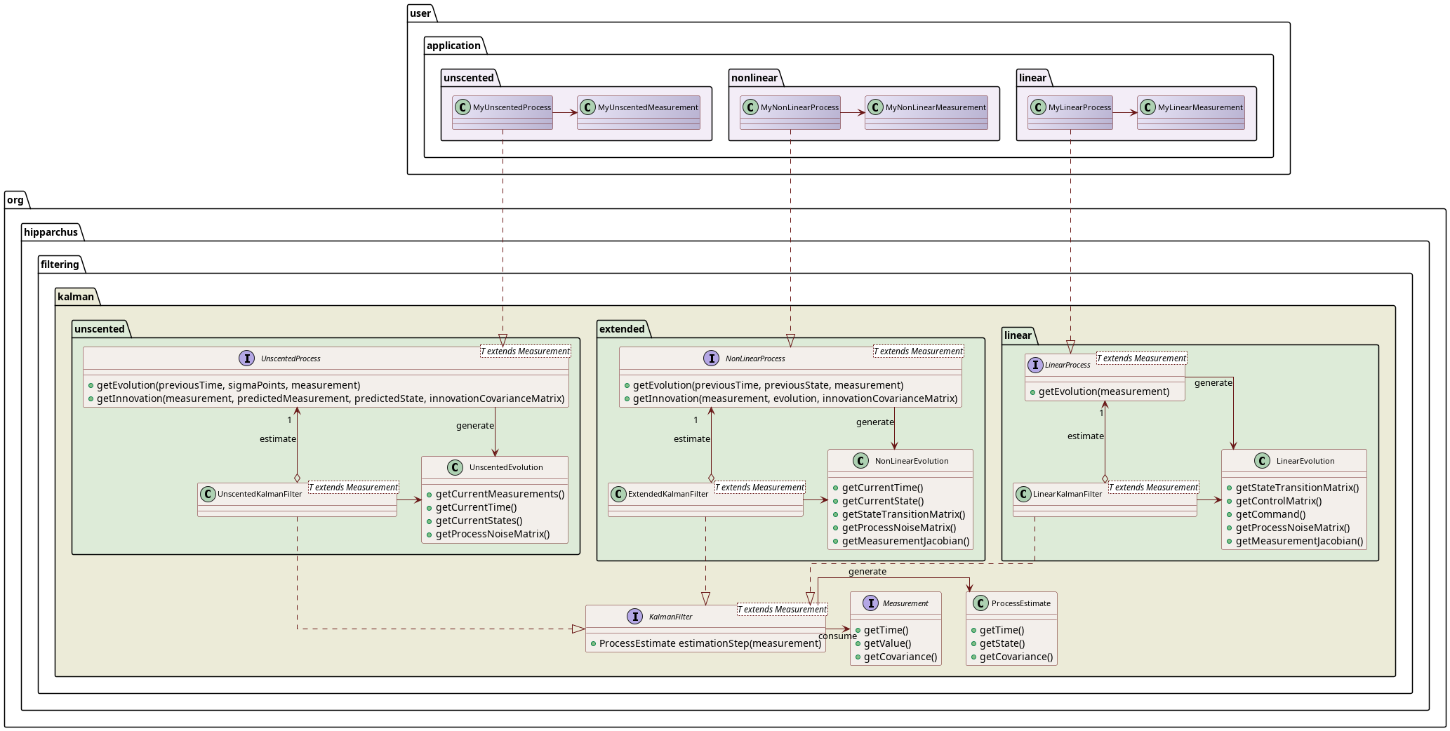
Kalman filters are devoted to real time estimates. They process measurements one by one as they arrive and produce a new estimate of the process state based on each measurement.
Depending on the type of process (linear or non-linear), a different type of Kalman filter should be used (see below), and different interfaces must be implemented by users to model their process.
In both cases, users must implement the general Measurement interface, and their implementation will be used as the parameterized type T in the filter.
In both cases, once users have created a Kalman filter of the appropriate type, they will feed it with measurements, getting back the process estimates, which correspond to the corrected values. If needed, the filter also stores the predicted values (as Kalman filter relies on a prediction/correction algorithm), so they can monitor precisely how the filter works.
In both cases, the user-implemented process can decide if a measurement should be completely ignored (typically if it is invalid or is an outlier). In this case, the correction phase is a no-op and the corrected process estimate will be the same as the predicted state estimate.
Linear processes
Linear processes with command are governed by the evolution equation on state \(x_k\):
\[ x_k = A_{k-1} x_{k-1} + B_{k-1} u_{k-1} + w_{k-1} \]
where
- \(A_{k-1}\) is the state transition matrix in the absence of control
- \(B_{k-1}\) is the control matrix
- \(u_{k-1}\) is the command
- \(w_{k-1}\) is the process noise, which has covariance matrix \(Q_{k-1}\)
and by the measurement equation on measurement \(z_k\): \[ z_k = H_k x_k + r_k \]
where
- \(H_k\) is the measurement matrix
- \(r_{k-1}\) is the measurement noise, which has covariance matrix \(R_k\)
In order to estimate the state of a linear process, users must implement the LinearProcess interface and create a LinearKalmanFilter instance.
If a measurement should be ignored, a null measurement Jacobian matrix should be put in the LinearEvolution instance returned by the linear process.
Non-linear processes
Non-linear processes with command are governed by the evolution equation on state \(x_k\):
\[ x_k = f(x_{k-1}) + w_{k-1} \]
where
- \(f\) is an evolution function
- \(w_{k-1}\) is the process noise, which has covariance matrix \(Q_{k-1}\)
and by the measurement equation on measurement \(z_k\): \[ z_k = m(x_k) + r_k \]
where
- \(m\) is a measurement function
- \(r_{k-1}\) is the measurement noise, which has covariance matrix \(R_k\)
In order to estimate the state of a non-linear process, users must implement the NonLinearProcess interface and create an ExtendedKalmanFilter instance.
If a measurement should be ignored, either a null measurement Jacobian matrix should be put in the NonLinearEvolution instance returned by the process, or a null innovation vector should be returned by the process. The former way can be used if the decision about ignoring the measurement can be taken early in the prediction phase, and the latter can be used when the decision needs to perform some computations based on the innovation covariance matrix. This second case typically occurs when rejecting outliers measurements is based on a ratio between the innovation (which is a residual) and the a posteriori measurement covariance. This avoids having a bad measurement pulling the process state very far from reality as the a priori measurement covariance included in the measurement itself can be very wrong.